Abstract

A protein’s structure is a key to understanding its function, which in turn is essential for any related biological applications. Protein folding is one of the most basic self-assembly processes in biology. Numerous different approaches to protein structure prediction exist, such as comparative modelling and fold recognition. Machine learning methods aim at designing a model to extract useful information and knowledge from biological databases. In our research, we used protein data bank as a database. Our sample consists of approximately 13,100 proteins. We used DSSP for the calculation of solvent accessible surface area (SASA). We used the molecular visualizing software Pymol for visualizing structures. We measured the correlation of average relative accessibility area (RSA) to the molecular weights or dipole moments for residues. We measured the correlation between sum of molecular weights and the sum of dipole moments in proteins. We measured the correlations between the average numbers of polar, nonpolar, and charged residues around buried polar residues and each of buried polar residue’s average of SASA, molecular weight, average RSA, and dipole moment. We reported many significant correlations, such as between nonpolar residues’ average of RSA and their molecular weights, and between buried polar residues’ average of RSA and the averages numbers of polar, charged, and nonpolar residues around buried polar residues.

Introduction

Understanding protein function is crucial to decipher disease etiology and discover new medicines. Experimental structure determination techniques are expensive, time consuming, applied only in specific domains of the protein and doesn’t work for large and complex proteins (Jiang, Xu et al. 2004). Protein function however is tied to its 3D structure (Jiang, Xu et al. 2004, Dill and MacCallum 2012).

Indeed, over the years, many scientists have conducted structure determination experiments in the form of X-Ray crystallography, NMR and cryo-electron microscopy experiments. The number of experimentally solved structures have grown dramatically. This abrupt increase in structures followed advances in next generation sequencing and other genomic shotgun approaches. Figure 1 shows the yearly growth of total structures deposited in the PDB from 1990 till 2017 (Protein Data Bank 2017).

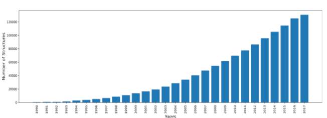
Figure 1: yearly growth of total structures deposited in the PDB from 1990 to 2017, drawn in python from PDB stats.

About 100,000 different kinds of protein may exist in a single living organism. Each protein has a primary sequence of amino acids linked by peptide bonds, which determines its unique folding conformation. Protein folding is the process by which a polypeptide chain folds into a specific, functional, stable, and three-dimensional structure(Dobson 2001, Onuchic and Wolynes 2004). The physical methods for protein folding entail solving how the physical driving forces interact with each other to promote the stable conformation among a huge number of possible conformations. The basic physical forces, which are responsible for protein folding, are hydrophobic interactions, van der Waals interactions, hydrogen bonding, and electrostatic interactions(Finkelstein and Galzitskaya 2004, Dill, Ozkan et al. 2008). Another used approach to utilize the huge amount of known protein sequences and structural data available in protein data bank is called “knowledge-based”. It is used to know the relation between protein sequences and folded structures(Chan, Kaya et al. 2002, Friesner, Prigogine et al. 2002). These statistics can be used in machine learning algorithms for classification and prediction.

Knowledge based structure prediction started early based on residue statistics of the propensity of certain residues to form or break certain secondary structures (Chou and Fasman 1978). This method was later improved by the GOR method which examines a window of seventeen residues, eight residues on each side of the residue being investigated, to either form or break a certain secondary structure (Garnier, Osguthorpe et al. 1978). Homology based modeling has gained a lot of popularity since then, and is the main basis for so many of the prediction methods that are used to date (Kumar and Singh 2016).

There are numerous research in the literature that conducted similar analysis on physico-chemical parameters of amino acid residues. JC Biro has investigated the top three physico-chemical parameters known to be involved in folding: the size, charge and hydrophobic moments of residues (Biro 2006). In his paper, he proved that compatible residues with similar physico-chemical parameters have a tendency to cluster together in 3D space. Another previous article has described significant correlation between the total protein’s molecular weight and it’s solvent accessible surface area (Janin, Miller et al. 1988). These findings are most intriguing and possibly suggest that such a relationship could exist at the residue level as well.

Like other knowledge based methods, our research takes advantage of the wealth of information in the Protein data bank. Indeed, knowledge based approaches have proven powerful at uncovering new pieces of evidence that fit the grand protein folding puzzle. Those little pieces of information, in fact, can make a very big contribution to improving the prediction accuracy (Kim, DiMaio, Wang, Song, & Baker, 2014). Specially by using machine learning, we can develop these pieces of information to efficient features, which can lead to good predicting models. Based on that one of the main important steps for building efficient models is choosing good features.

Tools and Methods

We used Python as our scripting language. We used many libraries and software packages to do our analysis. We used DSSP to calculate the solvent accessible surface areas (Kabsch & Sander, 1983; Touw et al., 2015) using the biopython Bio.PDB module (Cock et al., 2009; Hamelryck & Manderick, 2003). We used the molecular visualization software Pymol (Schrodinger, 2015) to visualize our structures. We used Matplotlib for plotting and visualizing, Scipy for statistical analysis, and Numpy for efficient operation on arrays.

We sampled our structures via the PDB advanced search tool. The choice of the structures were based on a few constraints that suit the purpose of our analysis. We excluded membrane proteins or proteins containing metals since these proteins have specific structures that affect the solvent accessibility surface area of residues. We restricted our choice to high quality structures based on XRay crystallography resolution between 0 and 3 Angstroms. The structures strictly had no ligands, modified residues and is not complexed with any RNA or DNA molecules. Our sample is comprised of approximately thirteen thousand and one hundred structures.

To conduct our analysis, we built a NOSQL database of JSON files for each PDB file containing the PDB ID, residue name, residue number, residue solvent accessible surface area. In order to visualize the parameters that we calculated, we constructed histograms of the solvent accessible surface areas. We divided the amino acids into charged, polar, and nonpolar (“The 20 Amino Acids: Hydrophobic, Hydrophilic, Polar And Charged Amino Acids”).

The relative solvent accessibility (RSA) was calculated for each amino acid by normalizing its accessible surface area by the maximum surface area by the reference values from Wilke (Tien, Meyer, Sydykova, Spielman, & Wilke, 2013). We measured the correlation between the average relative accessible surface areas and each residue’s molecular weight. In addition, we measured the correlation between the average relative accessible surface areas and each residue’s dipole moment(Khanarian and Moore 1980). The dipole moments are available for only 16 amino acids according to our reference.

We remarked during visualizing structures that there were some polar residues inside the protein interior but this was not expected as polar residues prefer being on the surface. Subsequently, We used residue’s RSA and a cut-off of 20%(Chen and Zhou 2005) to determine which polar residues are buried in each protein. By using Pymol, we selected the buried polar residues and counted polar, nonpolar and charged residues around them by 3 Å. We measured the correlation between the average of SASA for each residue and the average number of polar, nonpolar, and charged around it. We measured the correlation between molecular weight of each residue and the average number of polar, nonpolar, and charged around it. We measured the correlation between average RSA of each residue and the average number of polar, nonpolar, and charged around it. We measured the correlation between dipole moment of each residue and the average number of polar, nonpolar, and charged around it.

Finally, we measured the correlation between dipole moments of polar, nonpolar, and charged and their molecular weights. In addition, since we need a feature for proteins, we calculated the sum of molecular weights for each of polar, nonpolar, and charged in each protein. We calculated the sum of dipole moments for each of polar, nonpolar, and charged in each protein. We measured the correlation between the sum of molecular weights and the sum of dipole moments for each of polar, nonpolar, and charged as the protein is represented as a point on the graph.

Results

Figure 2 shows the correlation between molecular weights of charged residues and the average of RSA for each one on a sample of 13,100 proteins. The value of r square is 0.12 and the p value is 0.66 so there is no correlation. Figure 3 shows the correlation between dipole moments of charged residues and the average of RSA for each one on a sample of 13,100 proteins. The value of r square is 0.51 and the p value is 0.5 so there is a correlation but not significant as p value is bigger than 0.05. We expected this correlation since they carry a charge and they would favor polar interactions with water molecules, ions present inside the cellular environment and other polar residues.

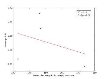
Figure 2: Molecular weights of charged residues is plotted against their average of RSA

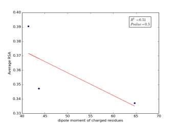
Figure 3: dipole moments of charged residues is plotted against their average of RSA

Figure 4 shows the correlation between molecular weights of polar residues and the average of RSA for each one on a sample of 13,100 proteins. The value of r square is 0.16 and the p value is 0.29 so there is no correlation.

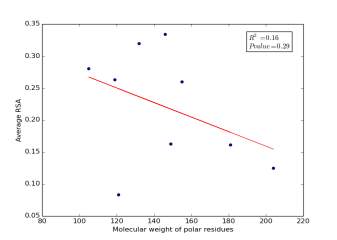
Figure 4: Molecular weights of polar residues is plotted against their average of RSA

Figure 5 shows the correlation between dipole moments of polar residues and the average of RSA for each one on a sample of 13,100 proteins. The value of r square is 0.24 so it is poorly correlated and the p value is more than 0.32 so this is not significant and there is no correlation. However, we notice in the two graphs that some polar residues are always near to each other so we expect that on we would find more relationships by doing more investigations on each group.

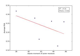
Figure 5: dipole moments of polar residues is plotted against their average of RSA

Figure 6 shows the correlation between molecular weights of nonpolar residues and the average of RSA for each one on a sample of 13,100 proteins. Figure 6a shows the correlation before removing the outlier point (Proline). The value of r square is 0.36 and the p value is 0.16 so this indicate that there is a poor correlation and not significant. Figure 6b shows the same relationship but after removing the outlier point. The correlation is stronger as the value of r square is 0.78 and it is high significant as the p value is 0.02.

a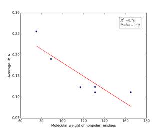  

b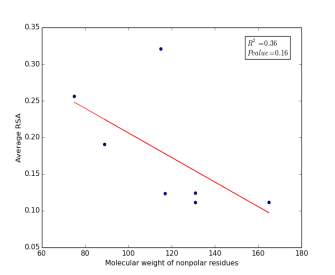

Figure 6: (a) Molecular weights of nonpolar residues is plotted against their average of RSA before removing the outlier point. (b) The same plot but after removing the outlier point.

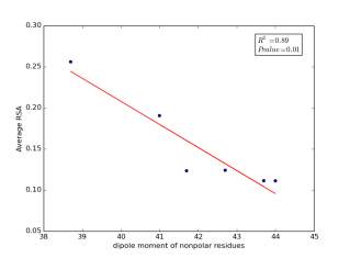
Figure 7 shows the correlation between dipole moments of nonpolar residues and the average of RSA for each one on a sample of 13,100 proteins. Figure 7a shows the correlation before removing the outlier point. The value of r square is 0.67 and the p value is 0.03 so this indicate that there is a significant correlation. Figure 7b shows the same relationship but after removing the outlier. The correlation is stronger as the value of r square is 0.89 and it is high significant as the p value is 0.01.

a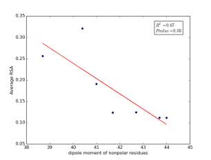 

b

Figure 7: a) dipole moments of nonpolar residues is plotted against their average of RSA before removing the outlier point. b) The same plot but after removing the outlier point.

As shown in figures 6 and 7, there are strong correlations between residues’ averages of RSA and both of their molecular weights and their dipole moments after removing Proline. Proline is a special case. Due to its ring side chain, it disrupts the peptide bond angle and introduces bends in the structure. It would then be expected for it to have more solvent exposure because of that. We found that 78% of nonpolar residues’ RSA variation is due to their molecular weights, and 89% of nonpolar residues’ RSA variation is due to their dipole moments. These correlations indicate that molecular weights and dipole moments have a role in protein folding for nonpolar residues. For further investigation, we should not study each variable individually but how they affect together on the solvent accessible surface areas by using multivariable models.

Figure 8 shows the correlation between the dipole moments of charged residues and their molecular weight. There is a high correlation as r square value is 0.82 but not significant as p value is 0.28. Thus, we cannot conclude that there is a correlation.

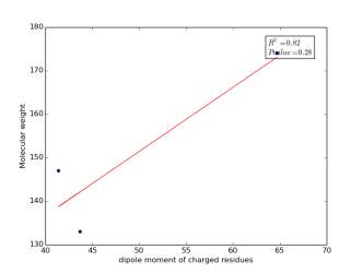
Figure 8: Dipole moments of charged residues are plotted against their molecular weights

Figure 9 shows the correlation between the dipole moments of polar residues and their molecular weights. There is no correlation as r square value is small and p value is 0.31.

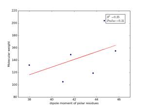
Figure 9: Dipole moments of polar residues are plotted against their molecular weights

Figure 10 shows the correlation between the dipole moments of nonpolar residues and their molecular weights. There is high significant correlation as the r square value is 0.75 and the p value is 0.01. These correlations in figures 6, 7, and 10 indicate that the combination of dipole moments and molecular weights plays a dominant role in determining the solvent accessible surface areas of nonpolar residues.

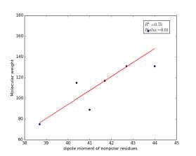
Figure 10: Dipole moments of nonpolar residues are plotted against their molecular weights

The relations showed in figures 8, 9, and 10 are characteristics of the amino acids not the proteins so we tried to represent these relations as features for proteins. Therefore, we calculate the sum of molecular weights for each of charged, polar, and nonpolar residues in each protein. We do the same for dipole moments. Finally, there are two numbers for each protein for each of charged, polar, and nonpolar residues.

Figure 11 shows the correlation between the sum of molecular weights for charged residues and the sum of dipole moments of them in each protein on a sample of 13.100 proteins so the point on the graph represents a protein. The value of r square is 1.0, which indicates that there are very strong correlation between them. The p value is 0.0 so this correlation is highly significant.

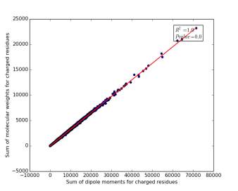
Figure 11: sum of dipole moments for charged residues is plotted against sum of molecular weights of them.

Figure 12 shows the correlation between the sum of molecular weights for polar residues and the sum of dipole moments of them in each protein. The value of r square is 0.99 that indicates that there are very strong correlation between them. The p value is 0.0 so this correlation is highly significant.

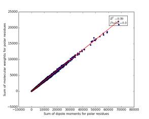
Figure 12: sum of dipole moments for polar residues is plotted against sum of molecular weights of them.

Figure 13 shows the correlation between the sum of molecular weights for nonpolar residues and the sum of dipole moments of them in each protein on a sample of 13.100 proteins so the point on the graph represents a protein. The value of r square is 1.0 that indicates that there are very strong correlation between them. The p value is 0.0 so this correlation is highly significant.

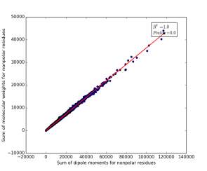
Figure 13: sum of dipole moments for nonpolar residues is plotted against sum of molecular weights of them.

Other very interesting relationships are shown in figures 11, 12, and 13. The three graphs show very high correlation. The more sum of molecular weights for polar, or nonpolar, or charged is, the more sum of dipole moments for them is. These correlations are high significant as the p value is very small, less than 0.05. This indicates we can use the total sum for dipole moments or molecular weights as a feature for predicting the other, respectively.

Figure 14 shows the correlation between averages of SASA for buried polar residues and averages of number of charged residues around them on a sample of 4000 proteins. The value of r square is 0.73 and the p value is approximately 0.0 so there is a strong correlation and it is high significant.

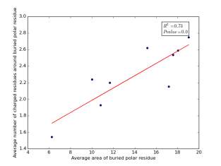
Figure 14: Plotting the averages of areas of buried polar residues against the averages of number of charged residues around them.

Figure 15 shows the correlation between the averages of RSA of buried polar residues and averages of number of charged residues around them on a sample of 4000 proteins. The value of r square is 0.93 and the p value is approximately 0.0 so there is a strong correlation and it is high significant.

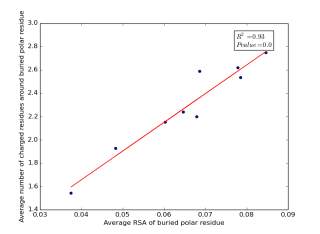
Figure 15: Plotting the averages of RSA of buried polar residues against the averages of number of charged residues around them.

We can conclude from figures 14 and 15 that the SASA or the RSA of buried polar residues plays a role in determining the number of charged residues around them during folding. Thus, we can use this feature to predict or confirm new protein structure. Machine learning models can further use these interesting relations to build good models to contribute to the protein folding problem.

Figure 16 shows the correlation between molecular weights of buried polar residues and averages of number of charged residues around them on a sample of 4000 proteins. The value of r square is 0.05 and the p value is 0.55 so there is no correlation.

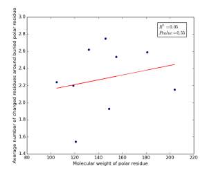
Figure 16: Plotting the molecular weights of buried polar residues against the averages of number of charged residues around them.

Figure 17 shows the correlation between dipole moments of buried polar residues and averages of number of charged residues around them on a sample of 4000 proteins. The value of r square is 0.04 and the p value is 0.69 so there is no any correlation. Thus, neither molecular weights nor dipole moments play a role in determining the number of charged residues around buried polar residues.

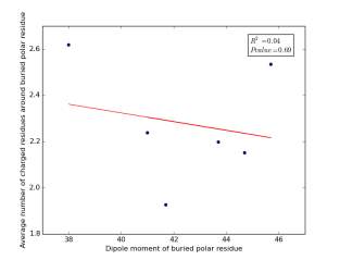
Figure 17: Plotting dipole moments of buried polar residues against the averages of number of charged residues around them.

Figure 18 shows the correlation between the averages of areas for buried polar residues and averages of number of nonpolar residues around them on a sample of 4000 proteins. The value of r square is 0.15 and the p value is 0.3 so there is no correlation.

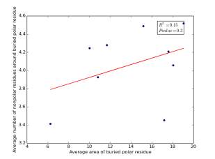
Figure 18: Plotting the averages of areas of buried polar residues against the averages of number of nonpolar residues around them.

Figure 19 shows the correlation between the averages of RSA for buried polar residues and averages of number of nonpolar residues around them on a sample of 4000 proteins. The value of r square is 0.68 and the p value 0.01 so there is a strong high significant correlation. We can conclude that SASA of buried polar residues does not play a role in determining the number of  nonpolar residues around them but the RSA can be used for predicting the number of nonpolar residues around them.

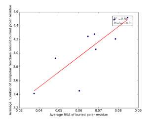
Figure 19: Plotting the averages of RSA of buried polar residues against the averages of number of nonpolar residues around them.

Figure 20 shows the correlation between the molecular weights for buried polar residues and averages of number of nonpolar residues around them on a sample of 4000 proteins. The value of r square is 0.14 and the p value 0.32 so there is no correlation.

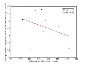
Figure 20: Plotting the molecular weights of polar residues against the averages of number of nonpolar residues around them.

Figure 21 shows the correlation between dipole moments for buried polar residues and averages of number of nonpolar residues around them on a sample of 4000 proteins. The value of r square is 0.27 and the p value 0.29 so there is no correlation. Thus, neither molecular weights nor dipole moments play a role in determining the number of nonpolar residues around buried polar residues.

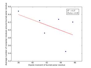
Figure 21: Plotting dipole moments of polar residues against the averages of number of nonpolar residues around them.

Figure 22 shows the correlation between the averages of areas for buried polar residues and averages of number of polar residues around them on a sample of 4000 proteins. The value of r square is 0.25 and the p value 0.18 so there is no correlation.

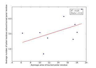
Figure 22: Plotting the averages of areas of buried polar residue against the averages of number of polar residues around them.

Figure 23 shows the correlation between the averages of RSA for buried polar residues and averages of number of polar residues around them on a sample of 4000 proteins. The value of r square is 0.54 and the p value 0.02 so there is a significant correlation. In addition, the RSA can be used for predicting the number of polar residues around buried polar residues.

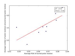
Figure 23: Plotting the averages of RSA of buried polar residues against the averages of number of polar residues around them.

Figure 24 shows the correlation between the molecular weights for buried polar residues and averages of number of polar residues around them on a sample of 4000 proteins. The value of r square is 0.02 and the p value 0.74 so there is no correlation.

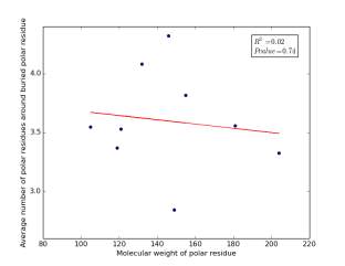
Figure 24: Plotting the molecular weights of buried polar residues against the averages of number of polar residues around them.

Figure 25 shows the correlation between the dipole moments for buried polar residues and averages of number of polar residues around them on a sample of 4000 proteins. The value of r square is 0.08 and the p value 0.59 so there is no correlation. As before, neither molecular weights nor dipole moments play a role in determining the number of polar residues around buried polar residues.

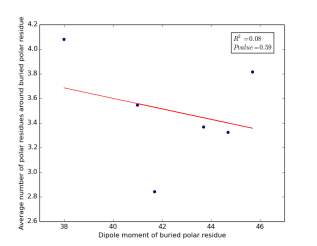
Figure 25: Plotting the dipole moments of buried polar residues against the averages of number of polar residues around them

Conclusion

In this paper, we establish a hierarchy for features involved in protein folding. As we showed, the molecular weight and the dipole moments play a significant role in the solvent exposure of hydrophobic residues. In addition, the relevant surface area plays a significant role in determining the number of residues around buried polar residues. To the best of our knowledge, this is a novelty and can achieve big contributions in protein structure prediction. By using these significant statistics in machine learning methods, we can build models for prediction. We can cluster the proteins into families and determine the percentage of correlation for each relationship mentioned above in each family. The combination of these percentages can then be used for prediction. Machine learning methods will continue to play a role in protein structure prediction. The growth in the size of the available training sets coupled with the gap between the number of sequences and the number of solved structures remain powerful motivators for further developments. Furthermore, machine learning methods are relatively fast compared to other methods in many cases. Both accuracy and speed considerations are likely to remain important as genomic, proteomic, and protein engineering projects continue to generate great challenges and opportunities in this area.

References

Biro, J. C. (2006). “Amino acid size, charge, hydropathy indices and matrices for protein structure analysis.” Theoretical Biology & Medical Modelling 3: 15-15.

Chan, H. S., H. Kaya and S. Shimizu (2002). “Computational methods for protein folding: scaling a hierarchy of complexities.” Current topics in computational molecular biology: 403-447.

Chen, H. and H.-X. Zhou (2005). “Prediction of solvent accessibility and sites of deleterious mutations from protein sequence.” Nucleic acids research 33(10): 3193-3199.

Chou, P. Y. and G. D. Fasman (1978). “Empirical predictions of protein conformation.” Annual review of biochemistry 47(1): 251-276.

Dill, K. A. and J. L. MacCallum (2012). “The protein-folding problem, 50 years on.” Science 338(6110): 1042-1046.

Dill, K. A., S. B. Ozkan, M. S. Shell and T. R. Weikl (2008). “The protein folding problem.” Annu. Rev. Biophys. 37: 289-316.

Dobson, C. M. (2001). “The structural basis of protein folding and its links with human disease.” Philosophical Transactions of the Royal Society of London B: Biological Sciences 356(1406): 133-145.

Finkelstein, A. and O. Galzitskaya (2004). “Physics of protein folding.” Physics of Life Reviews 1(1): 23-56.

Friesner, R. A., I. Prigogine and S. A. Rice (2002). Computational methods for protein folding, Wiley New York.

Garnier, J., D. J. Osguthorpe and B. Robson (1978). “Analysis of the accuracy and implications of simple methods for predicting the secondary structure of globular proteins.” Journal of molecular biology 120(1): 97-120.

Janin, J., S. Miller and C. Chothia (1988). “Surface, subunit interfaces and interior of oligomeric proteins.” Journal of molecular biology 204(1): 155-164.

Jiang, T., Y. Xu and M. Q. Zhang (2004). Current topics in computational molecular biology, Ane Books.

Khanarian, G. and W. Moore (1980). “The Kerr effect of amino acids in water.” Australian Journal of Chemistry 33(8): 1727-1741.

Kumar, R. and B. R. Singh (2016). Introduction to Protein Folding. Protein Toxins in Modeling Biochemistry. Cham, Springer International Publishing: 5-28.

Onuchic, J. N. and P. G. Wolynes (2004). “Theory of protein folding.” Current opinion in structural biology 14(1): 70-75.

Protein Data Bank. (2017). “Yearly Growth of Total Structures.” from http://www.rcsb.org/pdb/statistics/contentGrowthChart.do?content=total&seqid=100.

Bendell, C. J., Liu, S., Aumentado-Armstrong, T., Istrate, B., Cernek, P. T., Khan, S., . . .Murgita, R. A. (2014). Transient protein-protein interface prediction: datasets, features, algorithms, and the RAD-T predictor. BMC Bioinformatics, 15(1), 82. doi:

10.1186/1471-2105-15-82

Cock, P. J. A., Antao, T., Chang, J. T., Chapman, B. A., Cox, C. J., Dalke, A., . . . de Hoon, M. J. L. (2009). Biopython: freely available Python tools for computational molecular biology and bioinformatics. Bioinformatics, 25(11), 1422-1423. doi:

10.1093/bioinformatics/btp163

Eisenberg, D., Weiss, R. M., Terwilliger, T. C., & Wilcox, W.

(1982). Hydrophobic moments and protein structure. Paper presented at the Faraday Symposia of the Chemical Society.

Hamelryck, T., & Manderick, B. (2003). PDB file parser and structure class implemented in Python. Bioinformatics, 19(17), 2308-2310. doi:

10.1093/bioinformatics/btg299

Jiang, T., Xu, Y., & Zhang, M. Q. (2004). Current topics in computational molecular biology: Ane Books.

Kabsch, W., & Sander, C. (1983). Dictionary of protein secondary structure: pattern recognition of hydrogenbonded and geometrical features. Biopolymers, 22(12), 2577-2637.

Kim, D. E., DiMaio, F., Wang, R. Y.-R., Song, Y., & Baker, D. (2014). One contact for every twelve residues allows robust and accurate topology-level protein structure modeling. Proteins, 82(0 2), 208-218. doi:

10.1002/prot.24374

Miller, S., Janin, J., Lesk, A. M., & Chothia, C. (1987). Interior and surface of monomeric proteins. Journal of Molecular Biology, 196(3), 641-656.

Rost, B., & Sander, C. (1994). Conservation and prediction of solvent accessibility in protein families. PROTEINS: Structure, Function, and bioinformatics, 20(3), 216226.

Schrodinger, LLC. (2015). The PyMOL Molecular Graphics System, Version 1.8.

Tien, M. Z., Meyer, A. G., Sydykova, D. K., Spielman, S. J., & Wilke, C. O. (2013). Maximum Allowed Solvent Accessibilites of Residues in Proteins. PLOS ONE, 8(11), e80635. doi: 10.1371/journal.pone.0080635

Touw, W. G., Baakman, C., Black, J., te Beek, T. A., Krieger, E., Joosten, R. P., & Vriend, G. (2015). A series of PDBrelated databanks for everyday needs. Nucleic Acids Research, 43(D1), D364-D368.